Appendix F. Endnotes
Note 1. Making Resources Accessible
The appropriate technical expertise and resources may be located in house, but because of organizational structure, may not be readily accessible to a project managerAn individual from a regulatory agency (for example, federal, state, or local), or a consulting company, or responsible party company, who is coordinating the site cleanup including the risk assessment.. For example, this was the case in Texas. To support consistent implementation of risk-based corrective action programs and to maintain high caliber technical expertise, the technical experts housed in the various remediation programs were consolidated into one organizational unit so they could provide support to the project managers on an as-needed basis.
This effort achieved the goals of providing consistent and predictable expert support to the project managers via focused training, mentoring, and direct project support; allowed the agency to provide technical expertise and resources, but at the same time contain the expenses; fostered on-going program development and refinement; and helped to retain the technical experts over the long term.
See Section 3.1.1.2.
Note 2. Terms Describing Levels Below Which Concentrations are Reported
Various terms are used to describe the level below which concentrations are reported (for example reporting limit, detection limit, method detection limit, sample quantitation limit, instrument detection limit). There are differences in technical meanings, as presented in Section 5 of RAGS Part A (USEPA 1989a) and Section 5.7 of ITRC’s Groundwater Statistics and Monitoring Compliance (ITRC 2013). For a specific chemical, the value can vary by different characteristics (for example, laboratory, sample moisture content, other chemicals present in the sample).
See Section 4.5.4.1.
Note 3. When is route-to-route extrapolation from oral toxicity values not appropriate?
As stated in USEPA guidance (2009a), the following circumstances, included in the Inhalation Dosimetry Methodology (USEPA 1994b), are specific examples of situations when route-to-route extrapolation from oral toxicity valuesDerived values (for example, reference doses and slope factors) that can be used to estimate the incidence or potential for adverse human health effects in receptor (USEPA 2015h). might not be appropriate, even for use during screening:
- Groups of chemicals are expected to have different toxicity by the two routes – for example, metals, irritants, and sensitizers.
- A first-pass effect by the respiratory tract is expected.
- A first-pass effect by the liver is expected.
- A respiratory tract effect is established, but a dosimetry comparison cannot be clearly established between the two routes.
- The respiratory tract was not adequately studied in the oral studies.
- Short-term inhalation studies, dermal irritation, in vitro studies, or characteristics of the chemical indicate the potential for portal-of-entry effects at the respiratory tract, but studies themselves are not adequate for inhalation toxicity value development.
USEPA guidance (2009a) also provides more information about route-to-route extrapolation.
See Section 5.1.2.4.
Polycyclic Aromatic Hydrocarbons
- Toxicological Profile for Polycyclic Aromatic Hydrocarbons (PAHs) (ATSDR 1995).
- Provisional Guidance for Quantitative Risk Assessment of Polycyclic Aromatic Hydrocarbons (USEPA 1993b).
See Section 5.1.3.2.
Note 5. Using the RPF Approach for Cumulative Risk Assessments
- Organophosphorus Cumulative Risk Assessment – 2006 Update (USEPA 2006d).
- Triazine Cumulative Risk Assessment (USEPA 2006g).
- Cumulative Risk from Chloroacetanilide Pesticides (USEPA 2006a).
- Revised N-Methyl Carbamate Cumulative Risk Assessment (USEPA 2007d).
- Pyrethrins/Pyrethroid Cumulative Risk Assessment (USEPA 2011e).
See Section 5.1.3.2.
Note 6. Resources for Dioxins/Furans
- Recommended Toxicity Equivalence Factors (TEFs) for Human Health Risk Assessments of 2,3,7,8-Tetrachlorodibenzo-p-dioxin and Dioxin-Like Compounds (USEPA 2010d).
- Re-evaluation of Human and Mammalian Toxic Equivalency Factors for Dioxins and Dioxin-like Compounds (van den Berg et al. 2006).
- Adoption of Revised Toxicity Equivalency Factors (TEFWHO-05) for PCDDs, PCDFs, and Dioxin-like PCBs (CalEPA 2011).
See Section 5.1.3.3.
Polychlorinated biphenyls (PCBs)
- PCBs: Cancer Dose-Response Assessment and Application to Environmental Mixtures (USEPA 1996a).
See Section 5.1.3.3.
Note 8. CDC Concurrence Statement
The CDC defined this as: “We agree, but we do not have the funding, staff, or control over the means to implement the recommendation. The response highlights strategies that have been shown to be effective; however a commitment to implement actions cannot be made due to our lack of control over available resources” (CDC 2012a).
See Section 5.1.5.1.
Note 9. Range of Acceptable Lead Concentrations for Adult Exposure
As explained in USEPA (2003a) guidance, this range of soil lead concentrations derives from USEPA’s recommended default ranges for baseline BLL (PbB0 from 1.7 to 2.2 µg/dL) and geometric standard deviation (GSDi from 1.8 to 2.1), as summarized on Table 1 of the guidance. Specifically, USEPA derived the low end of the range (750 mg/kg) by using a GSDi of 2.1 and PbB0 of 2.2 µg/dL, and the high end of the range (1,750 mg/kg) by using a GSDi of 1.8 and PbB0 of 1.7 µg/dL.
See Section 5.1.5.2.
Note 10. USEPA Weight-of-Evidence Classifications
USEPA (2005b) presents the following classifications:
- carcinogenic to humans
- likely to be carcinogenic to humans
- suggestive evidence of carcinogenic potential
- inadequate information to assess carcinogenic potential
- not likely to be carcinogenic to humans
See Section 5.2.1.
In the case of some chemicals, consensus may not exist within the scientific and regulatory community regarding chemical classification. If consensus is not present, note this lack of agreement among experts in the Risk Characterization.
See Section 5.2.1.
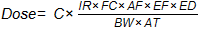
Where:
dose = mg chemical per kg body weight per day
C = chemical concentration (mg/L or mg/kg)
IR = intake rate (L/day or kg/day)
FC = fraction contacted (unitless)
AF = adsorbed fraction (unitless)
EF = exposure frequency (days/year)
ED = exposure duration (years)
BW = body weight (kg)
AT = averaging time (days)
Based on the equation in Exhibit 6-14 in Chapter 6 of USEPA's risk assessment guidance (USEPA 1989a).
See Section 6.1.
Note 13. Calculation of Inhalation Exposure Concentration
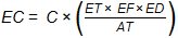
Where:
EC = time-weighted average concentration (mg/m3)
C = chemical concentration (mg/m3)
ET = exposure time (hours/day)
EF = exposure frequency (days/year)
ED = exposure duration (years)
AT = averaging time (hours)
Based on the equation in Exhibit 6-16 in Chapter 6 of USEPA's risk assessmentAn organized process used to describe and estimate the likelihood of adverse health outcomes from environmental exposures to chemicals. The four steps are hazard identification, dose-response assessment, exposure assessment, and risk characterization (Commission 1997a). guidance (USEPA 1989a).
See Section 6.1.
Note 14. Dose Calculation with Bioavailability Exposure Factor
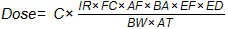
Where:
dose = mg chemical per kg body weight per day
C = chemical concentration (mg/L or mg/kg)
IR = intake rate (L/day or kg/day)
FC = fraction contacted (unitless)
AF = adsorbed fraction (unitless)
BA = bioavailability factor (unitless)
EF = exposure frequency (days/year)
ED = exposure duration (years)
BW = body weight (kg)
AT = averaging time (days)
Based on the equation in Exhibit 6-14 in Chapter 6 of USEPA's risk assessment guidance (USEPA 1989a and USEPA 2007c).
See Section 6.1.3.1.
Note 15. GIS Software for Polygons
An example of software that can be used to create Thiessen polygons is ESRI ARCGIS. In the ESRI ARCGIS software the Thiessen polygons can be generated by selecting ArcToolbox > Analysis Tools > Proximity > Create Thiessen Polygons (ESRI 2012).
See Section 6.2.4.2.
Note 16. Calculation of Area-weighted Average Concentrations
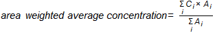
Where:
Ci = concentration at each individual sampling location
Ai = surface area (for example, acres) of the polygonal subarea constructed for each individual sampling location
See Section 6.2.4.2.
Note 17. States with Published Metals and PAH Background Data
Several states, including California, Illinois, Maine, Massachusetts, Michigan, New York, Ohio, and Washington have published background data for metals or PAHs in soil.
See Section 6.2.5.
Note 18. Segregation of Hazard Indices
For noncancer hazard indices, segregation of hazard indices by effect and mechanism of action may be appropriate (USEPA 1989a). This process can be complex and time-consuming because it is necessary to identify all of the major effects and target organs for each chemical and then to classify the chemicals according to target organ(s) or mechanism of action. This analysis is not simple and should be performed by a toxicologist. If the segregation is not carefully done, an underestimate of true hazard could result.
See Section 7.1.2.1.
Note 19. Example Forward and Backward Calculation
Basic Equation – Ingestion of Arsenic in Drinking Water - Adult
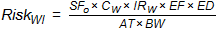
Where:
RiskWI = cancer risk for water ingestion (probability)
SFo = oral slope factorAn upper bound, approximating a 95% confidence limit, on the increased cancer risk from a lifetime exposure to an agent. This estimate, usually expressed in units of proportion (of a population) affected per mg/kg-day, is generally reserved for use in the low-dose region of the dose-response relationship, that is, for exposures corresponding to risks less than 1 in 100 (USEPA 2013). (1.5 [milligrams per kilogram-day]-1 or [mg/kg-
day]-1 for arsenic)
CW = concentration of chemical in water (milligrams per liter [mg/L])
IRW = ingestion rate (2 liters [L] per day for adults)
EF = exposure frequency (350 days/year)
ED = exposure duration (24 years for adult)
BW= body weight (70 kilogram [kg] adult)
AT = averaging time (70 years x 365 days/year; or 25,550 days)
Based on linear low-dose cancer risk equation presented in Section 8.2.1 and the equation in Exhibit 6-11 in Chapter 6 of USEPA's risk assessment guidance (USEPA 1989a).
Forward Risk Calculation
What is the risk of exposureContact of a receptor with a chemical. Exposure is quantified as the amount of the chemical available at the exchange boundaries of the organism (for example, skin, lungs, gut) and available for absorption (USEPA 1989a). to a specified arsenic concentration in groundwater?
- Assume arsenic concentration in groundwater, or CW is 0.001 mg/L. The only unknown in the equation is cancer risk which is calculated.
- For this example, cancer risk equals 1 x 10⁻⁵.
Backward Risk Calculation
What chemical concentration in groundwater (under the scenario above) would correspond to a cancer risk of one in a million or 1 x 10⁻⁶?
- Assume the cancer risk is 1 x 10⁻⁶. The only unknown in the equation is chemical concentration.
- For this example, the arsenic concentration in groundwater corresponding to a cancer risk of 1 x 10⁻⁶ is 0.000071 mg/L.
See Section 2.1.
Note 20. Lifetime Average Daily Dose Calculation for Drinking Water
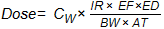
Where:
Dose = mg chemical per kg body weight per day
Cw = contaminant concentration (mg/L)
IR = ingestion rate (L/day)
EF = exposure frequency (days/year)
ED = exposure duration (years)
BW = body weight (kg)
AT = averaging time (days)
Based on the equation in Exhibit 6-11 in Chapter 6 of USEPA's risk assessment guidance (USEPA 1989a).
See Section 6.1.1.3.
Publication Date: January 2015